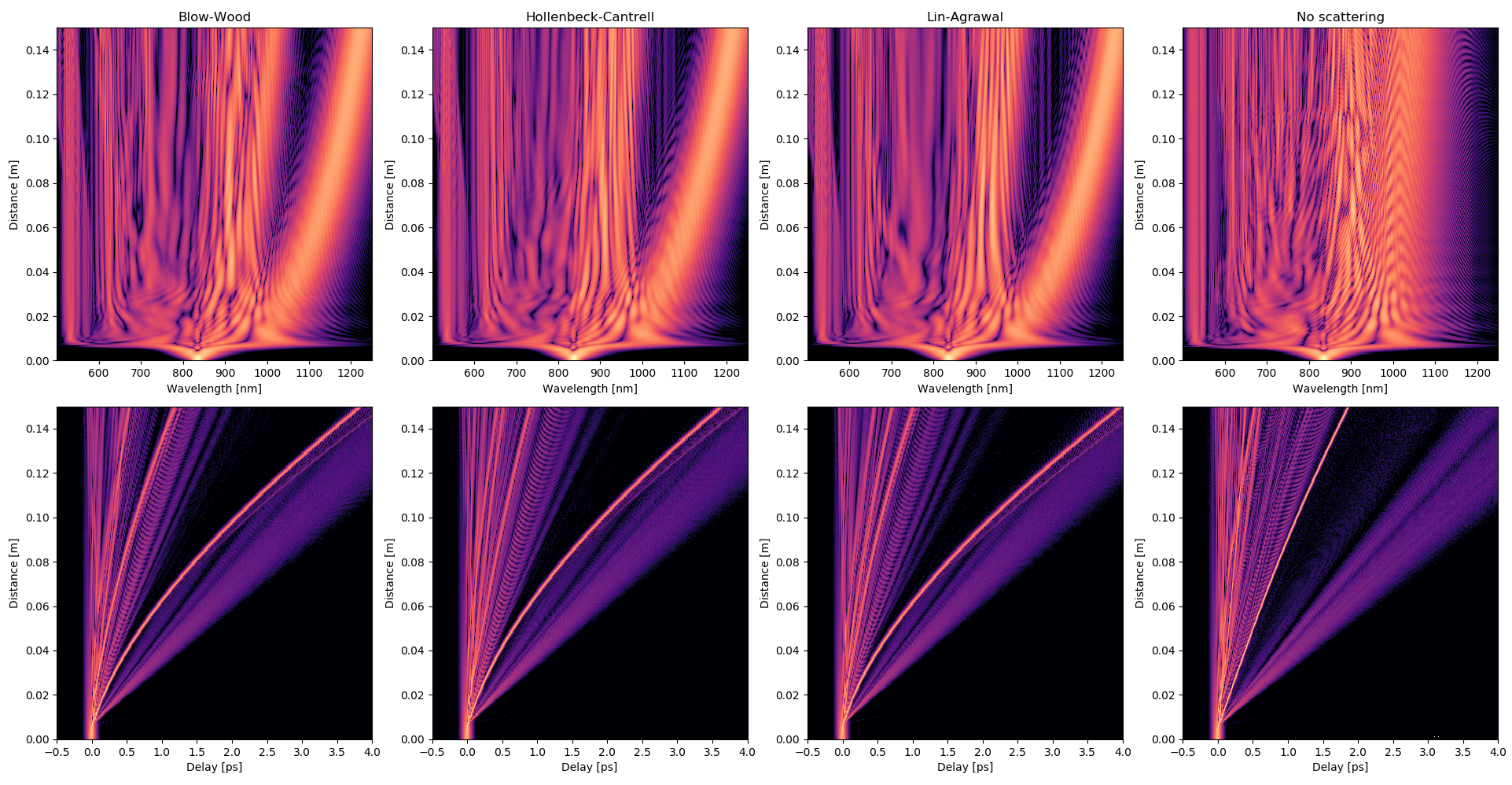
Dispersive wave generation in anomalous dispersion regime

Example of dispersive wave generation in anomalus dispersion regime at a central wavelength of 835 nm in a 15 centimeter long photonic crystal fiber using three different models to model Raman response.

import numpy as np
import matplotlib.pyplot as plt

import gnlse

if __name__ == '__main__':
    setup = gnlse.GNLSESetup()

    # Numerical parameters
    setup.resolution = 2**14
    setup.time_window = 12.5  # ps
    setup.z_saves = 400

    # Input pulse parameters
    peak_power = 10000  # W
    duration = 0.050284  # ps

    # Physical parameters
    setup.wavelength = 835  # nm
    setup.fiber_length = 0.15  # m
    setup.nonlinearity = 0.11  # 1/W/m
    setup.pulse_model = gnlse.SechEnvelope(peak_power, duration)
    setup.self_steepening = True

    # The dispersion model is built from a Taylor expansion with coefficients
    # given below.
    loss = 0
    betas = np.array([
        -11.830e-3, 8.1038e-5, -9.5205e-8, 2.0737e-10, -5.3943e-13, 1.3486e-15,
        -2.5495e-18, 3.0524e-21, -1.7140e-24
    ])
    setup.dispersion_model = gnlse.DispersionFiberFromTaylor(loss, betas)

    # This example extends the original code with additional simulations for
    # three types of models of Raman response and no raman scattering case
    raman_models = {
        'Blow-Wood': gnlse.raman_blowwood,
        'Hollenbeck-Cantrell': gnlse.raman_holltrell,
        'Lin-Agrawal': gnlse.raman_linagrawal,
        'No scattering': None
    }

    count = len(raman_models)
    plt.figure(figsize=(20, 10), facecolor='w', edgecolor='k')
    for (i, (name, raman_model)) in enumerate(raman_models.items()):
        setup.raman_model = raman_model
        solver = gnlse.GNLSE(setup)
        solution = solver.run()

        plt.subplot(2, count, i + 1)
        plt.title(name)
        gnlse.plot_wavelength_vs_distance(solution, WL_range=[500, 1250])

        plt.subplot(2, count, i + 1 + count)
        gnlse.plot_delay_vs_distance(solution, time_range=[-.5, 5])
    plt.tight_layout()
    plt.show()

Output: