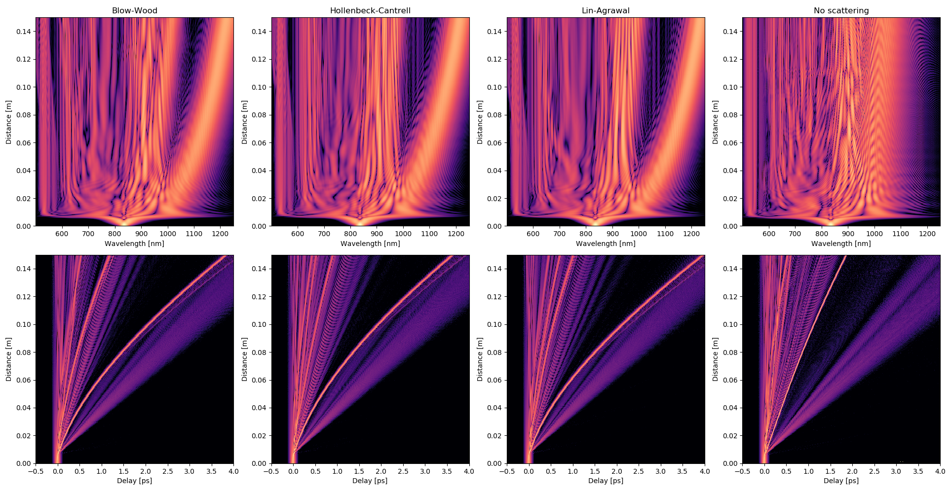
Dispersive wave generation in anomalous dispersion regime

Example of dispersive wave generation in anomalus dispersion regime at a central wavelength of 835 nm in a 15 centimeter long photonic crystal fiber using three different models to model Raman response.

import numpy as np
import matplotlib.pyplot as plt

import gnlse

import os

if __name__ == '__main__':
    setup = gnlse.GNLSESetup()

    # Numerical parameters
    setup.resolution = 2**14
    setup.time_window = 12.5  # ps
    setup.z_saves = 200

    # Physical parameters
    setup.wavelength = 835  # nm
    setup.fiber_length = 0.15  # m
    setup.nonlinearity = 0.0  # 1/W/m
    setup.raman_model = gnlse.raman_blowwood
    setup.self_steepening = True

    # The dispersion model is built from a Taylor expansion with coefficients
    # given below.
    loss = 0
    betas = np.array([-0.024948815481502, 8.875391917212998e-05,
                    -9.247462376518329e-08, 1.508210856829677e-10])

    # Input pulse parameters
    power = 10000
    # pulse duration [ps]
    tfwhm = 0.05
    # hyperbolic secant
    setup.pulse_model = gnlse.SechEnvelope(power, tfwhm)

    # Type of dyspersion operator: build from interpolation of given neffs
    # read mat file for neffs
    mat_path = os.path.join(os.path.dirname(__file__), '..',
                            'data', 'neff_pcf.mat')
    mat = gnlse.read_mat(mat_path)
    # neffs
    neff = mat['neff'][:, 1]
    # wavelengths in nm
    lambdas = mat['neff'][:, 0] * 1e9

    # Visualization
    ###########################################################################

    # Set type of dispersion function
    simulation_type = {
        'Results for Taylor expansion': gnlse.DispersionFiberFromTaylor(
            loss, betas),
        'Results for interpolation': gnlse.DispersionFiberFromInterpolation(
            loss, neff, lambdas, setup.wavelength)
    }

    count = len(simulation_type)
    plt.figure(figsize=(15, 7), facecolor='w', edgecolor='k')
    for (i, (name, dispersion_model)) in enumerate(simulation_type.items()):
        setup.dispersion_model = dispersion_model
        solver = gnlse.GNLSE(setup)
        solution = solver.run()

        plt.subplot(2, count, i + 1)
        plt.title(name)
        gnlse.plot_wavelength_vs_distance(solution, WL_range=[400, 1400])

        plt.subplot(2, count, i + 1 + count)
        gnlse.plot_delay_vs_distance(solution, time_range=[-.5, 5])

    plt.tight_layout()
    plt.show()

Output: