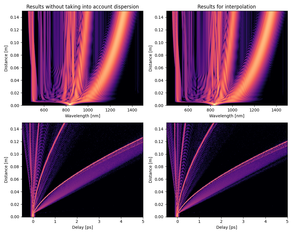
Consideration of mode profile dispersion
Consideration of mode profile dispersion in GNLSE account based on algorithm described in [J07]. Simulation conducted for a central wavelength of 835 nm in a 15 centimeter long photonic crystal fiber.
import matplotlib.pyplot as plt
import numpy as np
import os

import gnlse

if __name__ == '__main__':
    setup = gnlse.GNLSESetup()

    # Numerical parameters
    setup.resolution = 2**14
    setup.time_window = 12.5  # ps
    setup.z_saves = 200

    # Physical parameters
    setup.wavelength = 835  # nm
    w0 = (2.0 * np.pi * gnlse.common.c) / setup.wavelength  # 1/ps = THz
    setup.fiber_length = 0.15  # m
    setup.raman_model = gnlse.raman_blowwood
    setup.self_steepening = True

    # Input pulse parameters
    power = 1000
    # pulse duration [ps]
    tfwhm = 0.05
    # hyperbolic secant
    setup.pulse_model = gnlse.SechEnvelope(power, tfwhm)

    # The dispersion model is built from a Taylor expansion with coefficients
    # given below.
    loss = 0
    betas = np.array([-0.024948815481502, 8.875391917212998e-05,
                    -9.247462376518329e-08, 1.508210856829677e-10])
    setup.dispersion_model = gnlse.DispersionFiberFromTaylor(loss, betas)
    # parameters for calculating the nonlinearity
    n2 = 2.7e-20  # m^2/W
    Aeff0 = 1.78e-12  # 1/m^2
    gamma = n2 * w0 / gnlse.common.c / 1e-9 / Aeff0  # 1/W/m

    # read mat file for neffs to cover interpolation example
    mat_path = os.path.join(os.path.dirname(__file__), '..',
                            'data', 'neff_pcf.mat')
    mat = gnlse.read_mat(mat_path)

    # neffs
    neff = mat['neff'][:, 1]
    # wavelengths in nm
    lambdas = mat['neff'][:, 0] * 1e9
    # efective mode area in m^2
    Aeff = mat['neff'][:, 2] * 1e-12

    # This example extends the original code with additional simulations for
    nonlinearity_setups = [
        ["Scalar $\\gamma$",
        gnlse.DispersionFiberFromTaylor(loss, betas),
        gamma],
        ["Frequency dependent $\\gamma$",
        gnlse.DispersionFiberFromTaylor(loss, betas),
        gnlse.NonlinearityFromEffectiveArea(
            neff, Aeff, lambdas, setup.wavelength,
            n2=n2, neff_max=10)]
    ]

    count = len(nonlinearity_setups)
    plt.figure(figsize=(10, 8), facecolor='w', edgecolor='k')
    for i, model in enumerate(nonlinearity_setups):
        setup.dispersion = model[1]
        setup.nonlinearity = model[2]
        solver = gnlse.GNLSE(setup)
        solution = solver.run()

        plt.subplot(2, count, i + 1)
        plt.title(model[0])
        gnlse.plot_wavelength_vs_distance(solution, WL_range=[700, 1000])
        plt.subplot(2, count, i + 1 + count)
        gnlse.plot_delay_vs_distance(solution, time_range=[-.5, .5])

    plt.tight_layout()
    plt.show()
Output: