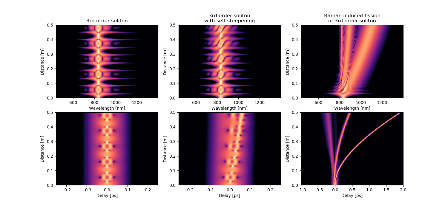
Propagation of higher-order soliton
Evolution of the spectral and temporal characteristics of the higher-order N = 3 soliton in three cases: - propagation without self steppening and Raman response; - soliton fission with self steppening, but no Raman response accounted; - soliton fission with self steppening, and Raman response accounted.
import numpy as np
import matplotlib.pyplot as plt

import gnlse

if __name__ == '__main__':
    setup = gnlse.gnlse.GNLSESetup()

    # Numerical parameters
    # number of grid time points
    setup.resolution = 2**13
    # time window [ps]
    setup.time_window = 12.5
    # number of distance points to save
    setup.z_saves = 200
    # relative tolerance for ode solver
    setup.rtol = 1e-6
    # absoulte tolerance for ode solver
    setup.atol = 1e-6

    # Physical parameters
    # Central wavelength [nm]
    setup.wavelength = 835
    # Nonlinear coefficient [1/W/m]
    setup.nonlinearity = 0.11
    # Dispersion: derivatives of propagation constant at central wavelength
    # n derivatives of betas are in [ps^n/m]
    betas = np.array([-11.830e-3])
    # Input pulse: pulse duration [ps]
    tFWHM = 0.050
    # for dispersive length calculation
    t0 = tFWHM / 2 / np.log(1 + np.sqrt(2))

    # 3rd order soliton conditions
    ###########################################################################
    # Dispersive length
    LD = t0 ** 2 / np.abs(betas[0])
    # Non-linear length for 3rd order soliton
    LNL = LD / (3 ** 2)
    # Input pulse: peak power [W]
    power = 1 / (LNL * setup.nonlinearity)
    # Length of soliton, in which it break dispersive characteristic
    Z0 = np.pi * LD / 2
    # Fiber length [m]
    setup.fiber_length = .5
    # Type of pulse:  hyperbolic secant
    setup.pulse_model = gnlse.SechEnvelope(power, 0.050)
    # Loss coefficient [dB/m]
    loss = 0
    # Type of dyspersion operator: build from Taylor expansion
    setup.dispersion_model = gnlse.DispersionFiberFromTaylor(loss, betas)

    # Set type of Ramman scattering function and selftepening
    simulation_type = {
        '3rd order soliton': (False, None),
        '3rd order soliton\nwith self-steepening': (True, None),
        'Raman induced fission\nof 3rd order soliton': (True,
                                                        gnlse.raman_blowwood)
    }

    count = len(simulation_type)
    plt.figure(figsize=(15, 7), facecolor='w', edgecolor='k')
    for (i, (name,
            (self_steepening,
            raman_model))) in enumerate(simulation_type.items()):
        setup.raman_model = raman_model
        setup.self_steepening = self_steepening
        solver = gnlse.GNLSE(setup)
        solution = solver.run()

        plt.subplot(2, count, i + 1)
        plt.title(name)
        gnlse.plot_wavelength_vs_distance(solution, WL_range=[400, 1400])

        plt.subplot(2, count, i + 1 + count)
        gnlse.plot_delay_vs_distance(solution, time_range=[-.25, .25])

    plt.tight_layout()
    plt.show()
Output: